Bayesian Inference for Quantum Error Correction
Overview
These two research projects used Bayesian statistical methods to perform error correction for quantum computers, as described in “A Logarithmic Bayesian Approach to Quantum Error Detection”:
We consider the problem of continuous quantum error correction from a Bayesian perspective, proposing a pair of digital filters using logarithmic probabilities that are able to achieve near-optimal performance on a three-qubit bit-flip code, while still being reasonable to implement on low-latency hardware. These practical filters are approximations of an optimal filter that we derive explicitly for finite time steps, in contrast with previous work that has relied on stochastic differential equations such as the Wonham filter. By utilizing logarithmic probabilities, we are able to eliminate the need for explicit normalization and can reduce the Gaussian noise distribution to a simple quadratic expression. The state transitions induced by the bit-flip errors are modeled using a Markov chain, which for log-probabilties must be evaluated using a LogSumExp function. We develop the two versions of our filter by constraining this LogSumExp to have either one or two inputs, which favors either simplicity or accuracy, respectively. Using simulated data, we demonstrate that the single-term and two-term filters are able to significantly outperform both a double threshold scheme and a linearized version of the Wonham filter in tests of error detection under a wide variety of error rates and time steps.
and “Machine Learning for Continuous Quantum Error Correction on Superconducting Qubits”:
Continuous quantum error correction has been found to have certain advantages over discrete quantum error correction, such as a reduction in hardware resources and the elimination of error mechanisms introduced by having entangling gates and ancilla qubits. We propose a machine learning algorithm for continuous quantum error correction that is based on the use of a recurrent neural network to identify bit-flip errors from continuous noisy syndrome measurements. The algorithm is designed to operate on measurement signals deviating from the ideal behavior in which the mean value corresponds to a code syndrome value and the measurement has white noise. We analyze continuous measurements taken from a superconducting architecture using three transmon qubits to identify three significant practical examples of non-ideal behavior, namely auto-correlation at temporal short lags, transient syndrome dynamics after each bit-flip, and drift in the steady-state syndrome values over the course of many experiments. Based on these real-world imperfections, we generate synthetic measurement signals from which to train the recurrent neural network, and then test its proficiency when implementing active error correction, comparing this with a traditional double threshold scheme and a discrete Bayesian classifier. The results show that our machine learning protocol is able to outperform the double threshold protocol across all tests, achieving a final state fidelity comparable to the discrete Bayesian classifier.
whose abstracts are given above.
The examples.ipynb notebook in the GitHub repo (linked above) provides a description of the Bayesian error correction algorithm, along with sample code that runs a toy example. The full model code can be found within the log_bayes.py and real_data.py modules in the src directory.
A non-interactive version of the Jupyter notebook is reproduced below.
A Brief Introduction to Quantum Error Correction
When using a quantum computer, we are interested in the behavior of objects known as qubits. A qubit is similar to the classical bit used in standard computers, except that it can take on states that are in-between the usual 0 and 1 binary values. These intermediate configurations are known as superpositions, and are what allow quantum computers to carry out certain tasks much more efficiently than standard computers.
One of the disadvantages of quantum computers is that they are very susceptible to errors. These errors perturb the state of the qubits, and will ultimately corrupt the output of the algorithm if not corrected. Fortunately, it is possible to monitor the state of the qubits in real time during a calculation and detect when an error occurs. An operation can then be performed on the affected qubit to undo the error and bring the qubit back into its correct state.
The qubits are monitored by performing quantum measurements, which will generate time-series data that can be analyzed to check for errors. The form of these measurements will change depending on the number of qubits and the type of errors that are expected, but for simplicity we will focus on a three-qubit system that is perturbed by bit-flip errors. Under normal operations, each qubit should be in the same state as the other qubits, but a bit-flip error on one of the qubits will break this symmetry. To determine which qubit has been flipped, we can perform a parity measurement on two different pairs of qubits, which gives a value of -1 if the two qubits are in the same state and +1 if they are in different states. If at least one measurement returns a value of +1, then we know that an error has occurred and can figure out which qubit was flipped.
The process described above is very straightforward if we can know the exact values of the parity measurements, but unfortunately this is often not possible. Instead, we end up with a signal whose mean will be centered on +1 or -1, but which will also have a large amount of Gaussian noise on top of it. To extract out the parity measurement, we must apply some kind of filtering algorithm to the signal, which is where Bayesian inference can be very useful.
The Measurement Data
Before describing the Bayesian model, we will first take a closer look at the measurement data itself. Since we are interested in training an algorithm to detect bit-flip errors, we will want to look at measurements from qubits that have been deliberately flipped in a consistent and controlled manner. The following code loads a set of sample measurement data and plots one of the time series:
import matplotlib.pyplot as plt
import numpy as np

data = np.load("src/data/measurements.npz")
measurements = data["measurements"][0, 1, :, 0] # Index 1 marks the qubit state, Index 2 marks the flipped qubit
print(f"The data has {measurements.shape[1]} measurements in the time series for each of the two qubit pairs.")
plt.plot(data["times"], measurements.T)
plt.xlabel(r"Time ($\mu$s)", fontsize = 16)
plt.ylabel("Measurement", fontsize = 16)
plt.gcf().set_size_inches(10, 7)
plt.show()
The data has 192 measurements in the time series for each of the two qubit pairs.
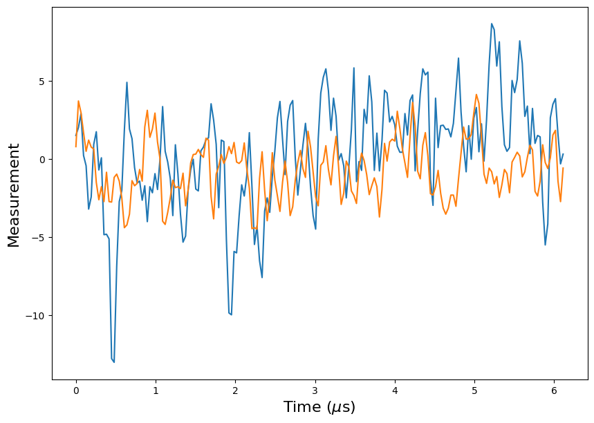
Although it is difficult to tell from this plot, both of the parity measurements (the parity of the first and second qubit is shown in blue, while the parity of the second and third qubits is shown in orange) are centered on -1 until the 3 \(\mu\)s mark. Then an error occurs on the first qubit, which causes the mean of the blue line to shift down to +1. It is clear from the plot that there is a significant amount of noise in the measurements, with noticeable autocorrelation between neighboring values.
Given the large variance in the measurements, the changes induced by the bit flips are easiest to see by plotting the measurement means.
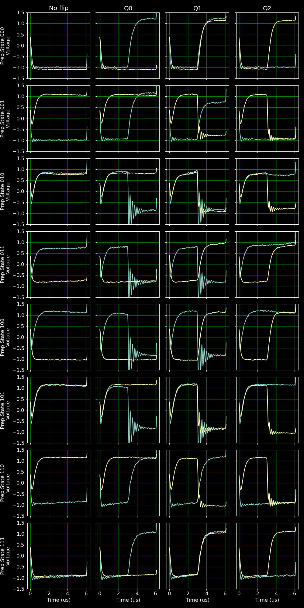
Each row of plots corresponds to a different starting configuration of the qubits, with each qubit either in the 0 or 1 state. The different columns correspond to different bit flips, with the first column containing no bit flips and columns 2, 3, and 4 corresponding to flips of qubits 1, 2, and 3 respectively. The figure as a whole shows several interesting behaviors, such as a clear oscillation pattern that occurs after certain flips. We can also see that the means do not exactly align at +1 and -1, but instead drift somewhat over time. These imperfections are something that will need to be dealt with by the filtering algorithm.
The Bayesian Filter
Our goal in quantum error correction is to determine what error, if any, has perturbed the state of the qubits in our quantum computer. Given the measurement signals plotted in the previous section, the detection of an error is equivalent to detecting when the mean of the measurement signal switches from -1 to +1. Assuming that the errors are uncorrelated, we can describe the system of qubits and measurement signals using a hidden Markov model. The qubit states represent a hidden Markovian variable, with a probability of transition depending only on the current state. Since the measurement signal follows a Gaussian distribution whose mean is determined by the qubit states, we can use observations of the signal to make inferences about the hidden Markov variable. The following code shows the basic features of the hidden Markov model:
import torch

class Bayesian():

    # This class represenrs the Bayesian classifier designed to handle
    # the autocorrelations present in imperfect measurement data.

    def __init__(self, depth):

        # The depth attribute determines how many prior syndrome measurements to
        # condition on when calculating the Gaussian likelihood of a new syndrome
        # measurement. For depth > 0, this allows the model to leverage any
        # autocorrelation that may be present in the data.

        self.depth = depth

        # This is simply a list of the other attributes that will be used.

        self.transition_matrix = None
        self.gauss_means = None
        self.gauss_precs = None
        self.prior = None
        self.prev_synd = None

    def classify(self, measurements):

        # This method returns the posterior probability, with shape (num_runs, 8),
        # of each label given a batch of measurments with shape (num_runs, 2). The
        # internal state of the classifier is also updated appropriately, with the
        # prior being updated to the posterior and the previous syndromes being
        # updated to include the new measurements.

        m_1_batch = torch.cat(
            [self.prev_synd[:, 0:1], measurements[None, 0:1]], dim=1)
        m_2_batch = torch.cat(
            [self.prev_synd[:, 1:2], measurements[None, 1:2]], dim=1)
        likelihood = self.get_gaussian_outputs(m_1_batch, m_2_batch)
        unnorm_probs = torch.einsum(
            "al,lr->ar", self.prior.float(), self.transition_matrix.float()) * likelihood
        posteriors = unnorm_probs / \
            torch.sum(unnorm_probs, dim=1, keepdim=True)
        self.prior = posteriors
        if self.depth:
            self.prev_synd = torch.cat(
                [self.prev_synd[1:, :], measurements[None, :]])
        return posteriors[0]

    def get_gaussian_outputs(self, m_1_batch, m_2_batch):

        # This method calculates the Gaussian likelihoods for the syndrome pair in
        # the most recent step, conditioned on a number of prior measurements determined
        # by the depth attribute. This means that the m_1_batch and m_2_batch must both
        # have shapes of (num_runs, depth + 1).

        (num_runs, num_steps) = m_1_batch.shape
        joint_batch = torch.cat([m_1_batch, m_2_batch], dim=1)
        marg_batch = torch.cat([m_1_batch[:, :-1], m_2_batch[:, :-1]], dim=1)

        joint_centered = joint_batch.reshape(
            [num_runs, 1, 2*(self.depth + 1)]) - self.joint_means.reshape([1, 8, 2*(self.depth + 1)])
        joint_expon = -0.5*torch.einsum("ali,lij,alj->al", joint_centered.float(
        ), self.joint_precs.float(), joint_centered.float())
        joint_output = joint_expon + 0.5*torch.slogdet(self.joint_precs)[1]

        if self.depth > 0:  # The marginal distribution only exists if depth > 0
            marg_batch = torch.cat(
                [m_1_batch[:, :-1], m_2_batch[:, :-1]], dim=1)
            marg_centered = marg_batch.reshape(
                [num_runs, 1, 2*self.depth]) - self.marg_means.reshape([1, 8, 2*self.depth])
            marg_expon = -0.5*torch.einsum("ali,lij,alj->al", marg_centered.float(
            ), self.marg_precs.float(), marg_centered.float())
            marg_output = marg_expon + 0.5*torch.slogdet(self.marg_precs)[1]
            log_output = joint_output - marg_output
        else:
            log_output = joint_output
        outputs = torch.exp(log_output)  # Only exponentiate at the end
        return outputs
The main method of interest here is classify, which takes as input two parity measurements (one for each pair of qubits) and returns a set of posterior probabilities for each qubit configuration (i.e. the state of the hidden Markov variable). The model starts by transforming its prior distribution, which are the probabilities generated by the previous call to classify (or the initial state of the qubits) using the bit-flip transition matrix, and then updates them based on the measurement data. Since the measurements are Gaussian distributed, we can easily compute the likelihood associated with each qubit state by setting the means to +1 or -1, which is done in the get_gaussian_outputs method. In order to take into account any autocorrelation between sequential samples, we can store the previous measurement values and use them as input to the Gaussian likelihood.
In the code block above, the transition matrix and Gaussian parameter are left uninitialized. To get values for them, we can fit to a set of measurement data like that shown in the previous section. For each qubit state, the means of the measurement values can be computed and stored in self.gauss_means, while variance and covariance values are stored in self.gauss_precs. The transition matrix cannot be fit using data with artificial errors, but its elements can be computed by assuming some plausible error rate for the quantum computer based on its hardware.
To evaluate a trained model, we can simulate measurement data and then test how well the model is able to predict the state of the (simulated) qubits. An example test is shown in the following code:
import torch

from src import tools, real_data

print("Generating data...")
(train_data, train_labels) = tools.Real_Simulated(error_rate_sec = 0.01*1e6).generate_data(30000, 60)
(test_data, test_labels) = tools.Real_Simulated(error_rate_sec = 0.01*1e6).generate_data(30000, 60)

model = real_data.Bayesian(0)
model.train(train_data, train_labels)

m_1 = test_data[:, :, 0]
m_2 = test_data[:, :, 1]
(num_runs, num_steps) = m_1.shape
outputs = torch.zeros([num_runs, 0])
model.prior = torch.zeros([num_runs, 8])
model.prior[torch.arange(num_runs), test_labels[:, 0].type(torch.long)] = 1
num_correct = torch.zeros([num_runs])
print("Testing...")
for step in range(num_steps):

    # For each step, the new prior is calculated by contracting the previous
    # prior with the transition matrix, then scaling by the measurement
    # probabilities.

    m_1_slice = m_1[:, step:step + 1]
    m_2_slice = m_2[:, step:step + 1]
    sample_probs = model.get_gaussian_outputs(m_1_slice, m_2_slice)
    unnorm_probs = torch.einsum("al,lr->ar", model.prior.float(), model.transition_matrix.float()) * sample_probs
    model.prior = unnorm_probs / torch.sum(unnorm_probs, dim = 1, keepdim = True)
    predictions = torch.argmax(model.prior, dim = 1)
    true_states = test_labels[:, step]
    fidelity = (predictions == true_states)
    num_correct = num_correct + fidelity
    outputs = torch.cat([outputs, predictions[:, None]], dim = 1)
    print("\rStep {}/{}".format(step, num_steps), end = "")

acc = num_correct * 100 / num_steps
print("\nAcc: {:.2f}%".format(torch.mean(acc)))
The final accuracy value reports how often the model correctly predicted the state of the system. Due to the irreducible noise in the measurement value, an accuracy of 100% will be virtually impossible for any large sample size. Indeed, the performance of this model is effectively optimal on the simulated data, since we use a Gaussian distribution to sample the measurement values and assume that the qubits states follow Markovian dynamics.